Star Detection
Everything Hocus Focus does (autofocus, the tilt/aberration inspector, sequence triggers) rests on one job: finding the real stars in a frame and measuring each one cleanly. The star detector takes a raw monochrome (or debayered) image and returns a list of accepted stars, each with a sub-pixel centroid, a local background, a Half-Flux Radius (HFR), and optionally a fitted PSF. It is deliberately conservative: the goal is not to count every point of light, but to keep a clean, well-measured set whose aggregate HFR is a trustworthy focus signal.
Why this detector is good
A naive "threshold and count blobs" detector is fooled by the things real astrophotos are full of: nebula and galaxy gradients, hot pixels, sensor noise, saturated cores, diffraction spikes, close double stars, and heavily defocused donuts. Hocus Focus addresses these head-on:
- Large-scale structure is removed before detection by subtracting an à-trous B3-spline wavelet residual, the coarse large-scale content that a multi-scale smoothing separates from star-sized structure, so nebulosity and sky gradients do not drown faint stars or create spurious blobs.
- The background is modeled as a tilted plane per star, not a single number, so a one-sided gradient under a star no longer biases its centroid, flux, or HFR.
- Contamination is detected even under a background gradient, so a neighboring star bleeding into one side of the measurement annulus is flagged and (by default) removed, instead of quietly corrupting the HFR.
- Multiple independent acceptance gates reject clipped, distorted, off-center, flat, dim, and contaminated candidates, each tracked as a named rejection count you can inspect.
- Aggregation is robust (median and median absolute deviation (MAD), plus an explicit outlier pass), so a handful of bad measurements cannot drag the reported focus metric around.
Nearly every stage is tunable. This page walks the pipeline in execution order; the Settings section documents each knob in detail, and the Optimization section can tune them for you against your own data.
The pipeline, in order
1. Region of interest (crop)
If a detection region smaller than the full frame is configured, the detector crops to that ROI first and applies all later stages inside it (an optional inner crop can additionally blank out a central region of the structure map). Working on a crop is faster and lets the inspector analyze sensor regions independently. The ROI offset is added back to every star's coordinates at the end, so positions are always reported in full-frame pixels.
2. Hot-pixel filtering
Single bright pixels (cosmic rays, sensor defects) look like tiny, intensely peaked stars and would survive most gates. A 3×3 median replaces a hot pixel with the median of its neighbors while leaving genuine stars (which span many pixels) essentially untouched. With Use Hotpixel Thresholding enabled, only pixels that exceed their surroundings by the configured threshold are corrected, so real star cores are preserved. For bayered images the filter runs on the raw CFA before debayering. See Hot Pixels & Saturation.
Note
Hot-pixel filtering also runs automatically whenever measurement noise reduction is enabled, because the blurring step would otherwise smear a hot pixel into a small false structure.
3. Noise reduction
An optional Gaussian blur (radius configurable) suppresses pixel-to-pixel noise so faint stars rise above the floor and the structure step is cleaner. It can be applied to the image actually measured, to the structure-detection copy only, or to neither. Blurring trades a little positional precision for sensitivity, so it helps most on noisy, short, or high-gain subs and can hurt on already-clean, well-sampled frames. See Preprocessing.
4. Wavelet structure detection (remove large-scale structures)
This step is what makes the detector insensitive to nebulae and gradients. The detector computes an à-trous B3-spline wavelet residual over a configurable number of layers and subtracts it, which removes structures larger than the stars while keeping the stars themselves. A short Gaussian smoothing then heals the holes that subtracting large scales can punch in the middle of big or out-of-focus stars.
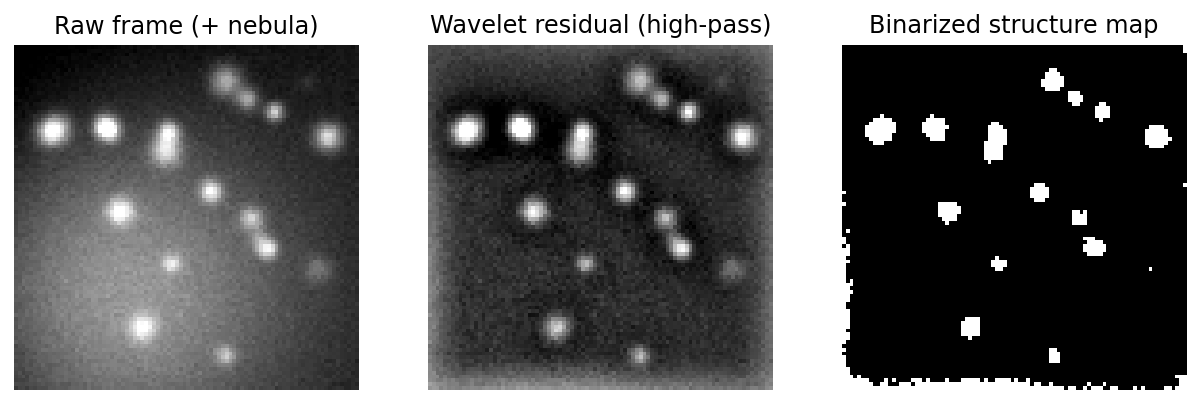
Left to right: the raw frame (with nebula), the wavelet residual capturing only star-scale structure, and the binarized structure map that defines candidate regions.
The number of structure layers is the key knob: too few and large or defocused stars get cut away with the nebula; too many and the background creeps back in. At very small pixel scales, or when you need a wide defocus range, more layers help. An opt-in defocus-aware mode adds extra layers via a boost so bloated donut stars survive the subtraction. See Structure Detection.
5. Binarization (noise floor)
The smoothed structure map is thresholded into foreground (star) vs. background. The threshold is the structure map's median plus the Noise Clipping Multiplier times an estimated noise sigma, where the sigma comes from a Kappa-Sigma noise estimate (an iterative clip-at-k·σ robust estimate) on the noise-reduced image:
Raising \( k_\sigma \) demands a stronger signal to count as a star (fewer, more reliable detections); lowering it admits fainter structure (more stars, more risk of noise). By default this threshold is computed per region rather than once for the whole frame (locally adaptive binarization), so the same multiplier stays fair across a vignetted or gradient-heavy frame. See Preprocessing, and Adaptive Binarization for how the local surface keeps a single multiplier fair everywhere.
6. Optional dilation
A morphological dilation (ellipse element, configurable size and iteration count) can grow the binarized foreground slightly. This boosts small structures and bridges narrow gaps so a single star is not split into fragments. Dilation is off by default (Structure Dilation Iterations is 0) and is most useful when stars are barely resolved. See Structure Detection.
7. Connected-component candidate boxes
The detector scans the binarized map and floods each connected foreground region into a candidate, recording its bounding box and pixel list. Every candidate is collected here with no size or shape filtering — the gates come next. The running total is reported as the structure candidates count, the denominator for all the rejection statistics.
8. Per-candidate measurement
For each candidate the detector measures, in order:
- Local background plane. Pixels in an annulus around the star (the bounding box expanded by a configurable margin) are fit to a tilted plane \( b_0 + b_1\,dx + b_2\,dy \) by robust iteratively reweighted least squares with Huber weights. This models a smooth one-sided gradient (galaxy, nebula, bright neighbor halo) instead of assuming a flat background. The plane is then subtracted per pixel everywhere it matters (centroid, flux, and HFR), so a gradient no longer biases the measurement. On a flat field the plane equals the annulus median, so nothing changes.
- Centroid. An iterative flux-weighted centroid; after the first pass it restricts contributing pixels to a circular aperture around the running estimate, so bright off-axis pixels do not pull the center of an asymmetric or tilted star.
- HFR. The flux-weighted mean radius over the star's circular aperture, sampled on a grid through the centroid with the background plane subtracted at each sample. This is the primary focus quantity.
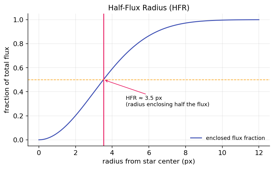
HFR is the radius of the aperture containing half the star's flux, a focus-sensitive size measure that does not require fitting a model.
The pixel sampling step controls the HFR grid: a finer step samples undersampled stars more faithfully at some cost in speed. See Preprocessing and PSF Modeling for the optional model fit (step 10).
9. Acceptance gates
Each measured candidate must clear every gate to be accepted. Each gate is also a named rejection counter, so the metrics panel tells you exactly why candidates are being dropped:
| Gate | Rejects when | Tune with |
|---|---|---|
| Too small | bounding box width or height below the minimum box size | Min Bounding Box Size |
| On border | bounding box touches a frame edge (likely clipped) | — |
| Too distorted | fill ratio (pixels / \(d^2\)) below the max-distortion threshold | Max Distortion |
| Degenerate | parameters could not be computed | — |
| Low sensitivity | normalized brightness / noise sigma at or below the sensitivity threshold | Brightness Sensitivity |
| Not centered | centroid falls outside the centered acceptance sub-box | Star Center Tolerance |
| Too flat | star median at or above peak-response × peak (a flat blob, not a peaked star) | Star Peak Response |
| HFR failed / too low | HFR could not be measured, or is at/below the minimum HFR | Min HFR |
| Contaminated | a one-sided neighbor was detected in the annulus (when rejection is on) | Contamination Sensitivity |
The fill-ratio idea behind too distorted: a round disk fills about \( \pi/4 \approx 0.79 \) of its bounding box, while a streak (a satellite trail or merged pair) fills far less. The Defocus-Aware Gates option (opt-in) relaxes the distortion and centering gates for large candidates so bloated donut stars near the sweep extremes are not thrown away; with it off, detection is unchanged. For telescopes with a central obstruction, the separate opt-in Recover Out-of-Focus Donut Stars group goes further, reconnecting fragmented hollow rings and treating them like filled disks so they survive at all. Full per-gate detail lives in Acceptance Gates.
Saturated stars are kept, not rejected
A partially-saturated star (background + peak at or above the saturation threshold) is not rejected. It is tracked in the saturation metric, and if PSF modeling runs, its clipped core pixels are masked during the fit rather than discarding the star. See Hot Pixels & Saturation.
Gradient-robust contamination test
The contamination test reuses the robust background plane from step 8: it subtracts the fitted plane from the annulus pixels, splits the residuals into eight angular sectors, and flags the star only when a single sector shows a one-sided positive residual excess above the contamination-sensitivity threshold (scaled by a local, MAD-based noise estimate). Because a contaminant adds light, the test ignores both smooth gradients (already removed by the plane fit) and edge-clip deficits, which are negative.
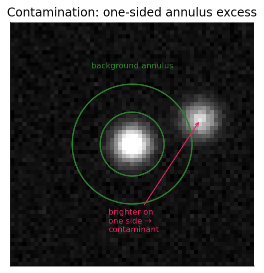
A neighboring star brightens one side of the annulus. The plane fit absorbs smooth gradients; a one-sided positive bump in a single sector is what trips the contamination flag.
By default, contaminated stars are rejected so the HFR and PSF statistics stay clean; you can instead keep and merely flag them (used by the diagnostics tooling). See Contamination.
10. Optional PSF modeling
When enabled (off during autofocus, where speed matters), each accepted star is fit with a Gaussian or Moffat point-spread function in parallel. A fit is accepted only if its \( R^2 \) meets the goodness-of-fit threshold; otherwise it is counted as a PSF failure and the star keeps its empirical HFR. The PSF yields sigma, FWHM in arcseconds, and eccentricity, the shape metrics the tilt/aberration inspector relies on. See PSF Modeling and the Tilt / Aberration Inspector overview.
11. Outlier rejection and aggregation
The surviving stars are aggregated into the frame-level numbers. By default the detector reports the median HFR (robust to a few bad measurements). In the mean-with-outlier-rejection mode it first computes the median and MAD, then discards stars outside
before averaging the rest. PSF-derived sigma, FWHM, and eccentricity are likewise aggregated by median and MAD across the stars that fitted successfully. The result is one clean HFR (and shape) value per frame, the signal that autofocus and the inspector consume.
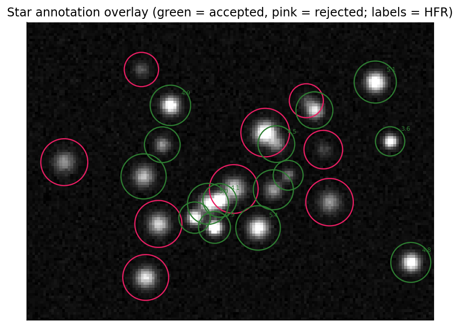
The final accepted set (green) versus rejected candidates (pink), each labeled with its HFR. This overlay is what the annotator draws on the image.
Where to go next
- Tune any stage: the Settings section has one page per pipeline area.
- Let the plugin tune detection against your own focus runs: Optimization.
- See the data behind the detector's key defaults: Precision & Recall.
- See how the accepted stars are drawn on the image: Star Annotation.