Sensor Model Fitting
The Tilt & Aberration Inspector turns a focus sweep into numbers for tilt, field curvature, and backfocus. Those numbers come from fitting a surface to where best focus falls across the sensor. This page covers that surface: the two models the inspector fits, how the measurements that feed them are gathered, the weighted fit itself, how outliers are detected and dropped, and the features that keep the result trustworthy.
This is the math companion to that inspector page, which covers the panel, its readouts, and the options that choose which model runs and tune it. Both models are built from focus curves measured by the same engine as a normal Autofocus run. The 4-corners model uses one best-focus position per region (the center and four corners); the sensor surface model uses one per star, each fit with the hyperbola family from Hyperbolic Curve Fitting.
Throughout, \(x\) and \(y\) are sensor positions in microns measured from the image center, and \(z\) is the focuser position (in microns) at which that point of the sensor reaches best focus.
Two models, one surface
The inspector fits the focus surface at two levels of detail.
- The 4-corners model (the tilt plane on the inspector page) is the simpler of the two, always computed. It measures best focus at the center and the four corners, then reads tilt from how the corners differ and backfocus from how the corners sit relative to the center. It is cheap and needs only those five focus curves, but it cannot tell field curvature apart from backfocus, and it says nothing about sensor centering.
- The sensor surface model (the Sensor Curve Model Enabled option) is the rigorous model. It fits a focus curve for every matched star across the frame, then fits a tilted paraboloid through all of those best-focus positions. That extra data lets it separate tilt, field curvature, and centering, and put an uncertainty on each result. It is also more demanding: it needs many well-fit stars, so it is more sensitive to measurement error and does not always succeed.
The two are not rivals. The 4-corners model captures only the linear part of the focus surface: drop the curvature terms from the paraboloid and you are left with the same kind of tilt plane. It is enough for a quick corner-versus-center check. The surface model is what you want when you intend to correct the sensor physically: a successful fit measures tilt, field curvature, and centering independently, so you can address each systematically. Correct tilt with differential screw moves. The wizard reads the field curvature as a spacing error and derives a backfocus correction from it, applied by moving all the adapter screws together (or adding spacers); the curvature that remains at the optimal spacing is the optical residual you can only minimize.
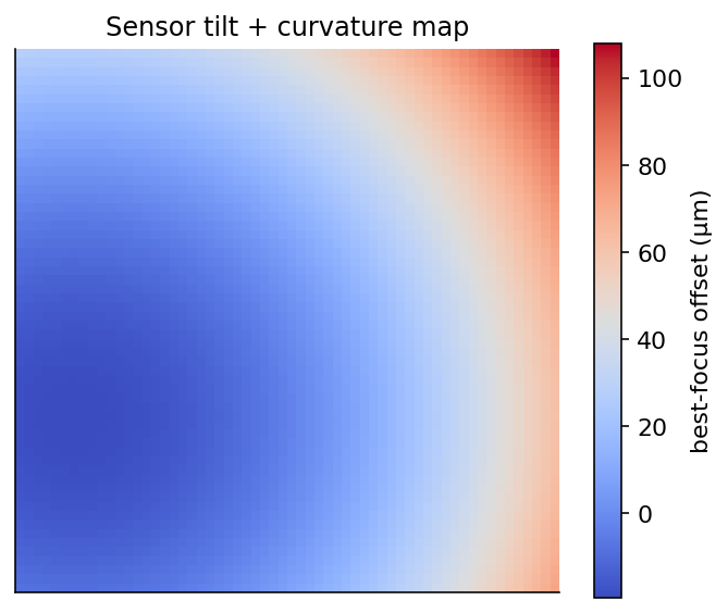
Best focus is reached at a different focuser position across the sensor. A smooth left-to-right gradient is tilt; a center-to-corner bowl is curvature. The models below separate the two.
The 4-corners model
The center and four corner regions each yield an estimated best-focus position. The center is held back for the backfocus comparison below; the four corners are fed to an ordinary-least-squares fit of a plane, over normalized image coordinates that run from \(-0.5\) to \(+0.5\) on each axis:
\(A\) and \(B\) are the tilt slopes along the horizontal and vertical axes (in focuser steps per normalized image unit) and \(C\) is the mean focus plane. Each corner's required adjustment (the Adj Steps / Adj Microns columns) is its best-focus position minus that mean, reported in focuser steps (and in microns when Focuser Step Size is set). There is no outlier rejection here, because there are only four points to fit.
Backfocus is read off the same regions rather than the plane: it is the mean of the four corner best-focus positions minus the center position, converted to microns with Focuser Step Size, and compared against the critical focus zone. A positive value means the corners reach focus at a higher focuser position than the center. With Increasing focuser position left at its default, that means the sensor sits too far from the corrector, and the panel says so: Move sensor TOWARDS flattener. Set that option to reversed and the same reading points the other way (see which way does your focuser travel). The screw-by-screw guidance built from this plane is covered under Guiding tilt-adapter screw adjustments.
The sensor surface model
The surface model fits a tilted paraboloid:
Each parameter has a physical reading:
- \(G_x, G_y\) are the tilt gradients, the change in best-focus position per micron of sensor displacement. They are the linear (planar) part of the surface.
- \(K_x, K_y\) are the curvature coefficients. They bow the surface into a bowl or dome.
- \(X_0, Y_0\) locate the optical center (the vertex of the paraboloid) relative to the image center, so a decentered field can be modeled rather than mistaken for tilt.
- \(Z_0\) is the focuser position of the surface at its center.
By default the field is modeled as rotationally symmetric: \(K_x = K_y = K\), one curvature coefficient and six free parameters. Turning on Astigmatic field curvature lets \(K_x\) and \(K_y\) differ, a seventh parameter that represents the saddle-shaped field of an astigmatic optical train. Leave it off unless you have reason to expect astigmatism, since the extra parameter is easier to over-fit.
The inspector also reports the familiar tilt and curvature quantities, derived from the fitted parameters:
\(\theta\) is the tilt angle and \(\varphi\) its direction. The linear-gradient form above replaces an older parameterization written directly in \((\theta, \varphi, K)\); writing the surface as a linear function of \(G_x, G_y, K_x, K_y\) removes a numerical trap at zero tilt (where the tilt direction is undefined) and lets the curvature cross zero, so a single fit covers a bowl, a dome, and a flat field without special cases.
The fit also yields a tilt plane in the same form as the 4-corners model above: the planar part of the surface evaluated at the four sensor corners. It carries the pixel pitch it was fit at, so the Tilt Adapter Wizard, which reads the plane's slopes back as microns of focuser travel per micron of sensor displacement, uses the pitch of the frames the plane came from rather than the camera profile's unbinned value. A calibration measured at 2x2 binning therefore recovers the same hardware numbers as one measured at 1x1.
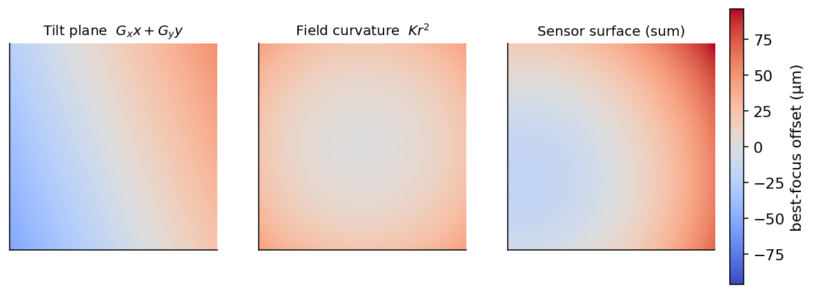
The surface is a tilt plane plus a curvature term. The fit estimates both at once and reports them separately, so you can tell a tilt problem (fixable with screws) from field curvature (an optical property of the corrector and focal ratio).
From stars to data points
Each data point in the surface fit is one star's best focus. Getting there takes three steps.
Per-star focus curves. Every star is tracked across the sweep (the cross-frame matching is described under registration below), and its HFR-versus-focuser-position points are fit with a hyperbola. The fit gives the star's best-focus position and its standard error \(\sigma\) (how sharply that position is pinned down). A star whose curve fit explains less than \(R^2 = 0.90\) of its own variation, or fails to fit at all, is discarded rather than contributing a noisy point.
Cross-frame registration. Stars drift in pixel position from frame to frame as the image breathes through focus, so they have to be matched into tracks before any star's curve can be fit. Matching itself is done with a k-d tree of nearest neighbors: the stars of a reference frame seed a registry, and each other frame's stars are matched to it by nearest neighbor within a search radius. The reference is the frame with the most detected stars, so the registry and the frame alignment have as many anchor stars as possible to match against.
Two registration approaches are available, set by Align images before matching (on by default) under Inspector options:
- Nearest-neighbor only (alignment off). Stars are matched directly in their original pixel positions, using a wide search radius so the frame-to-frame drift still falls inside it.
- RANSAC alignment first (alignment on). Every frame is first transformed onto the reference frame by a RANSAC-estimated transform (a similarity transform by default, or an affine one when Use affine alignment (diagnostic) is on), so matching stars land almost on top of each other. The nearest-neighbor match then runs with a much tighter search radius. This is what keeps matching reliable at the defocused ends of the sweep, where stars are bloated and sparse.
A frame that does not align to the reference on the first pass is retried against a denser set of reference triangles, and can also be matched to its nearest already-aligned neighbor, whose similar defocus makes its stars easier to match than the sharp reference. A frame stays unplaced when it is defocused enough that its few stars sit too far apart to form the small triangles the RANSAC step matches on. For that frame, and for a dense copy of the reference, the aligner then rebuilds the triangles over a larger box. The box grows by about half each step, up to roughly a third of the shorter image dimension, until the frame forms enough triangles to estimate a transform. A plate-scale check rejects any transform that would not keep the frame at close to its original scale, so a chance match cannot register a frame wrongly. These retries run only for frames the first pass could not place, and the box escalation triangulates only the brightest stars (about 120 of them), so a dense field, which aligns on the first pass, is neither altered nor slowed. If any frame still cannot be placed, star matching for the whole sweep reverts to the wider nearest-neighbor search radius used when alignment is off.
A frame whose star detection comes back empty (an extreme-defocus end of the sweep, a frame lost to cloud) does not stop the analysis. It stays in the run but contributes nothing: with no stars it has nothing to match and forms no triangles, so it never aligns. With alignment on, it therefore counts toward the "N frames failed to align" line that drops the whole sweep back to the wider search radius, and the inspector warns about it separately as well: "N frame(s) had no detected stars and were skipped". The remaining frames fit the model normally. If every frame in the run is empty there is no reference frame to register against, and the analysis fails with a message that says so ("Sensor modeling failed. None of the … frames in this run had any detected stars."). Longer exposures, or more sensitive star detection settings, are the fix.
A star must be matched in at least five frames to be fit, so its focus curve has enough points to be meaningful.
Building the points. Each surviving star contributes one data point: its sensor position in microns, \(\bigl((\text{pixel} - \tfrac{W}{2})\cdot p,\ (\text{pixel} - \tfrac{H}{2})\cdot p\bigr)\) for pixel size \(p\), and its best-focus position in microns. \(p\) is the pitch of the frames as they were captured: the camera pixel size from the frame's own metadata, multiplied by the binning the frame was taken at. A sweep captured with NINA's Auto Focus Binning at 2x2 uses twice the native pitch, so the sensor's physical size still comes out right. Detection Binning does not enter it, because the detector reports star positions back in the captured frame's pixels. The point carries the per-star uncertainty \(\sigma\), which becomes the fit weight
A tightly-pinned star pulls on the fit harder than a loosely-pinned one. When a star's \(\sigma\) is unavailable it is filled in with the median \(\sigma\) of the other stars, so an unknown uncertainty is treated like a typical star rather than dominating or being ignored. Every \(\sigma\), imputed or not, then gets a 2-micron floor added in quadrature. A per-star curve fit can report a formal standard error far below the real star-to-star scatter, and without that floor a handful of stars would carry nearly all of the fit's weight.
Fitting the surface
The surface is fit by weighted nonlinear least squares (Levenberg–Marquardt), minimizing the weighted sum of squared residuals
which is the \(\chi^2\) of the fit when \(w_i = 1/\sigma_i\). The model is linear in every parameter except the center \((X_0, Y_0)\), and the model's gradient is supplied analytically rather than estimated by finite differences, which makes the fit faster and more stable. The same per-point weight is applied to the residuals and to the gradient, so the optimizer's step stays consistent with what it is minimizing.
Two details keep the fit well-behaved:
- Parameter scaling. The parameters span very different magnitudes (a center offset in microns, a dimensionless gradient near \(10^{-3}\), a curvature coefficient near \(10^{-6}\)). The optimizer is told each parameter's scale so it can take sensible steps in every direction at once.
- The center. With Sensor Centered on (the default), \(X_0\) and \(Y_0\) are pinned to zero and the sensor is assumed centered. Turning it off lets the fit estimate the center along with everything else, bounded to the sensor's own dimensions. Pinning the center is more than an optics assumption: a free center and the tilt gradients are partly confounded (a small shift of the vertex looks like a little tilt), so fixing it also tightens the remaining parameters and their error bars.
Detecting and rejecting outliers
A bad star (a blend, a hot pixel mistaken for a star, a cosmic ray) can land far from the true surface. The model rejects outliers at three levels, from the individual measurement up to the whole surface.
Within a star's focus curve. With the inspector's Outlier rejection on (the default), a star's own HFR points are screened with a Grubbs test on the median- and MAD-scaled residuals before its best focus is trusted, and the star is refit without the point that fails. How many points the screen may drop is capped by the AutoFocus Max Outlier Rejections setting, which is 0 out of the box, so no point is dropped until you raise it. Under the default Hybrid (Best Fit) model each candidate curve proposes its own outliers and only the points every one of them flags are removed, so no curve can win the model comparison by pruning its own data. The screen never prunes a star below five points.
Across the surface. After the surface is fit, every point's weighted residual is measured (its distance from the surface divided by its own \(\sigma\), the quantity the fit minimizes) and the spread of those residuals is summarized robustly with the scaled median absolute deviation
where the constant makes the MAD a consistent estimate of the standard deviation for clean Gaussian scatter. Any point that lands more than \(2.5\,\operatorname{MAD}\) from the median residual is dropped and the surface is refit on what remains. This repeats until a pass drops nothing, capped at ten passes and at a tenth of the points in total. That cap is the backstop: rejection is there to remove a few bad stars, so once more than 10% of the data looks like an outlier the pruning stops rather than trimming the data into agreeing with the model.
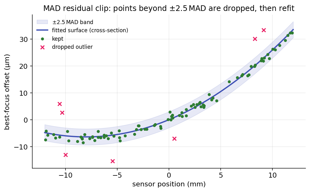
Most stars scatter tightly around the fitted surface. The few that fall outside the \(\pm 2.5\,\operatorname{MAD}\) band are dropped, then the surface is refit, so a handful of bad star measurements cannot pull the tilt and curvature off true.
The MAD is used instead of the standard deviation on purpose. The MAD has a 50% breakdown point, so a cluster of gross outliers cannot inflate the spread enough to hide themselves, which is exactly the failure mode of clipping on the standard deviation.
What makes the fit robust
A few additional safeguards keep the result stable from run to run.
- Inverse-variance weighting lets confident stars carry the fit and noisy ones step aside, with median imputation so a missing uncertainty neither dominates nor disappears.
- Minimum data requirements. At least nine stars are needed to fit a surface at all, each star needs five matched frames, and the inspector warns when fewer than ten stars made it into the model.
- An overfit guard. A fit that explains the data almost perfectly (\(1 - R^2 < 0.005\)) is treated as suspicious rather than excellent, since on this kind of data it usually means too few points survived to constrain the surface.
- A deliberate acceptance gate. A low \(R^2\) on its own never rejects the model, because a nearly flat sensor genuinely explains little variance while still being fit well. The model is rejected only when \(R^2\) is below Min R² (rejection) (default \(0.05\)) and the reduced \(\chi^2\) is also poor (above \(5\)).
- Determinism. The per-star curve fits run in parallel but are written back in a fixed order, so the surface fit, and every number derived from it, is identical no matter how the work was scheduled.
Fit-quality metrics
Four numbers describe how well the surface fits the points and how precisely it pins the parameters.
| Metric | What it measures |
|---|---|
| \(R^2\) (weighted) | Fraction of the best-focus variation the surface explains. Reported as the model fit quality; low values only reject the model alongside a poor reduced \(\chi^2\). |
| Reduced \(\chi^2_\nu\) | Weighted residuals relative to the per-star error bars. Independent of how tilted the sensor is, which is what makes it a repeatable acceptance criterion. |
| RMS error | Plain (unweighted) root-mean-square residual, in microns. An intuitive "how far off, typically." |
| Std errors | One-sigma uncertainties on the tilt angle and the curvature radius. |
Reduced chi-squared is the \(\chi^2\) per degree of freedom,
with \(n\) enabled points and \(p\) the model's parameter count (six, or seven with Astigmatic field curvature on; a pinned center still counts here, unlike in the covariance below). Because the per-star \(\sigma\) is an approximate uncertainty rather than a calibrated one, \(\chi^2_\nu\) routinely runs above 1 even for good fits and its absolute scale depends on the rig, which is why it only rejects a model in combination with a low \(R^2\).
The error bars come from the fit covariance. At the solution the parameter covariance is
with \(J\) the model's Jacobian, \(W = \operatorname{diag}(w_i^2)\), and \(f\) the number of free parameters (a pinned center is excluded, so it cannot make the matrix singular). The tilt angle and curvature radius are functions of the parameters, so their uncertainties follow by the delta method. For the radius the relation is simple: \(R \propto 1/|K|\), so its relative error equals the curvature coefficient's, \(\sigma_R / R = \sigma_K / |K|\). When the fit is rank-deficient or ill-conditioned, or the field is so flat that the radius diverges, the standard error is reported as not determined rather than as a misleading finite number.
From fit to physical numbers
The fitted parameters are converted into the quantities the panel displays.
| Result | How it is computed |
|---|---|
| Tilt | The angle \(\theta = \arctan\sqrt{G_x^2 + G_y^2}\), in degrees, with its one-sigma error. |
| Tilt effect | Half the spread of the planar term across the four sensor corners: the worst-case best-focus offset, in microns, caused purely by tilt. |
| Curvature radius | \(R = 1 / (2000\,\lvert K \rvert)\) millimeters. Larger is flatter (and better), with its one-sigma error. |
| Curvature effect | The curvature term evaluated at a corner: the corner-to-center offset, in microns, caused purely by field curvature. |
| Critical focus | \(\text{CFZ} = 2.44\,F^2 \cdot 0.55\) microns, from the telescope focal ratio \(F\). The tolerance the other effects are graded against. |
| Centering | The optical-center offsets \(X_0, Y_0\); flagged when either exceeds ten pixels. |
| Mean focuser position | The focuser position that minimizes total defocus over the whole surface, from the surface's mean elevation (a closed-form integral of the paraboloid over the sensor). |
| AutoFocus offset | The mean focuser position minus the autofocus result, in steps: how far a single center-of-frame autofocus lands from the surface's best compromise. |
The grading uses the critical focus zone as the yardstick. Tilt is called acceptable when its effect is within \(0.25 \times \text{CFZ}\); curvature when its effect is within \(1.5 \times \text{CFZ}\). A tilt adapter removes the tilt (linear) part with differential screw moves, and reduces the curvature effect by moving all screws together to change the backfocus spacing (see the Tilt Adapter Wizard); the curvature that remains at the optimal spacing is a property of the corrector and focal ratio, addressed with a better-matched corrector or stopping down rather than the adapter. The direction of those all-screws moves comes from the adapter-direction setting (or the wizard's optional direction measurement); if the backfocus guidance seems inverted, flip that setting.